Please note that this is not an interactive notebook. However, you can run the binder yourself under the following link:
https://mybinder.org/v2/gh/MikeJSPerry/ESA_CCI_LST_DEMO/HEAD
Find the LST_cci data description here:
https://climate.esa.int/en/projects/land-surface-temperature
Python script with example analysis of LST_cci data
Authors: Michael Perry and Karen Veal (University of Leicester)
Import the relevant python modules required for the example: xarray and matplotlib
import xarray as xr
import numpy as np
import matplotlib.pyplot as plt
import pandas as pd
from SubRoutines.indexing import find_matching_index
from SubRoutines.plotting import lccs_manger
Specify the file to read in. In this case we are reading LST derived from MODIS AQUA, the data has been process to L3 and therefore has been reprojected to a regular grid (0.25 degrees in this example):
esacci_lst_025 = "Data/ESACCI-LST-L3C-LST-MODISA-0.25deg_1MONTHLY_DAY-20060701000000-fv3.00.nc"Open file using xarray (xr), the file will be read into a dataset (ds) structure:
ds = xr.load_dataset(esacci_lst_025)We can display the data within the dataset easily:
ds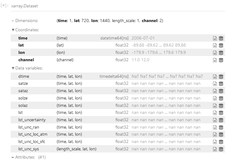
We can also plot the lst data directly (size and aspect are added here to make the image larger, but are not required):
ds.lst.plot(aspect=2,size=8)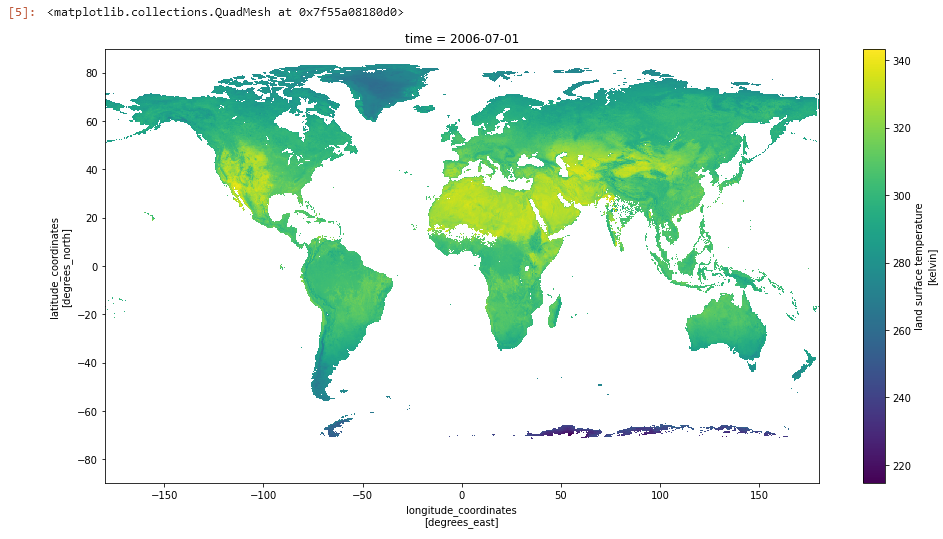
We can also look at the global distribution of LST:
ds.lst.plot.hist(size=8,bins=50, alpha=0.5, color='steelblue',edgecolor='grey')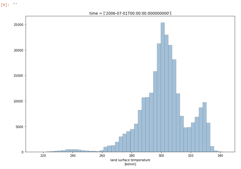
And we can look at specifc regions, first lets set our region of interest:
lower_lon = 105.0
upper_lon = 145.0
lower_lat = 25.0
upper_lat = 65.0
Next we find the indexes in the dataset which bound this region:
lat_max_idx = find_matching_index(ds.lat.values,upper_lat)
lat_min_idx = find_matching_index(ds.lat.values,lower_lat)
lon_max_idx = find_matching_index(ds.lon.values,upper_lon)
lon_min_idx = find_matching_index(ds.lon.values,lower_lon)
Ready to go. First we use “slice” to cut our the region of interest for both the lat and lon determined by the indexes we just determined. Then the plotting code is updated to use this region:
lat_region = slice(lat_min_idx, lat_max_idx)
lon_region = slice(lon_min_idx,lon_max_idx)
ds.lst.isel(lat=lat_region,lon=lon_region).plot(aspect=2,size=8)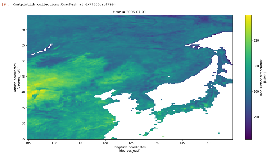
We can also run for transects. Similar to the region subsetting above, we specify at latitute, then find the corresponding index in the array and plot all longitudes at that latitude:
lat_transect = 50.0
lat_idx = find_matching_index(ds.lat.values, lat_transect)
ds.lst.isel(lat=lat_idx).plot(aspect=2,size=8)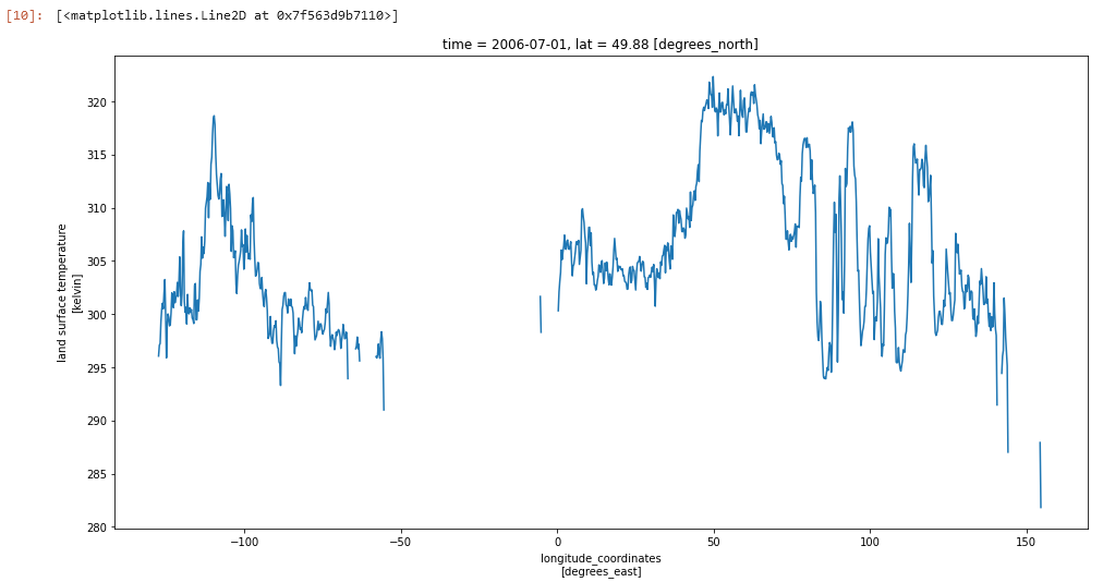
We can also explore some of the other paramters provided with the LST CCI data by looking at another product. Here we will use some 0.01 degree MODIS AQUA data that has been regridded to a subset (lat: 40–>45, lon: 117–>122):
esacci_lst_001 ="Data/ESACCI-LST-L3C-LST-MODISA-0.01deg_1MONTHLY_DAY-20220901103756-fv3.00.nc"
regridded_ds = xr.open_dataset(esacci_lst_001)

regridded_ds.lst.plot(aspect=2,size=8)
plt.title(f"time = {np.datetime_as_string(regridded_ds.time.values[0],unit='M')}")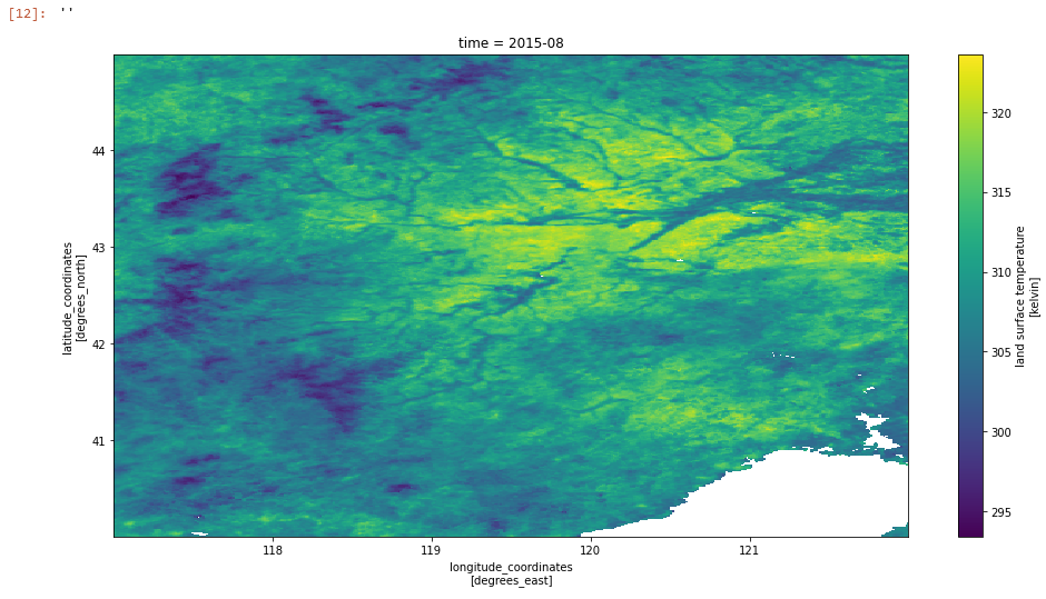
The data contains several variables that were not in the 0.25 degree data such as land cover classification (lcc):
lccs_data = lccs_manger(regridded_ds)
lccs_data.analyse_region()
lccs_data.plot_map()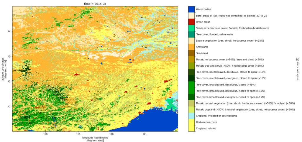
We can inspect the corresponding values of these classes in the attributes:
regridded_ds.lcc.attrs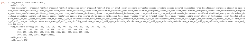
We can also inspect the distribution of these lccs:
Note the plot currently displays as a percentage cover of the region interest. If you would prefer the raw number of pixels in each class change “percentage=True” to “precentage=False”.
lccs_data.plot_distribution(percentage=True)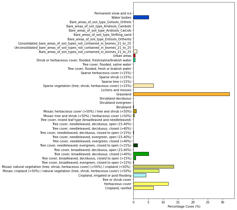
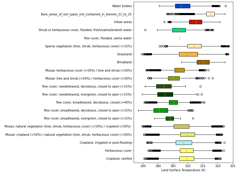
This can be correlated against LST to see the lcc distribution of temperature.
lccs_data.bin_lst_by_lcc()
lccs_data.box_plot()